Convert Jupyter Notebooks into Functions

Parameterize notebooks so you can programmatically run them

You’ve trained your machine learning model in a Jupyter notebook. Now, you want to run that model on data that comes in daily.

Day in, day out, you create a new copy of the same notebook and run it. You store the copy of the notebook and pass that results to your stakeholders.

In another scenario, you have a new set of data every day that needs to be visualized with the same code on Jupyter notebook.

So, you create a new copy of the same notebook and modify the input. Again, you store the copy of the notebook and pass the results to your stakeholders.

Doesn’t that sound painful?

That could be solved if we could have a function run_notebook(input_data). By providing the parameterinput_data, the notebook would run with the new input_data. The output would be a copy of the notebook run with the new data.

That is exactly what Papermill does.

Here’s a quick demo of what it does.

Papermill: Parameterize and execute Jupyter notebooks automatically

It is an open-sourced tool for parameterizing, executing, and analyzing Jupyter notebooks. Just pass in parameters to the notebook, and the Jupyter notebook runs automatically.

Use cases of Papermill

Running the same analysis on multiple data sets is time-consuming and error-prone if done manually. For example, a daily reporting dashboard might need to be refreshed on new data daily. Papermill automates this.

Machine learning algorithms in Jupyter notebooks might be used to generate results daily. Instead of manually running the notebook with fresh data daily, Papermill can be used to generate results in production.

In this post, I go through:

• Install Papermill
• Get started with Papermill
• Generate a visualization report regularly with Papermill
• Run machine learning algorithm in production with Papermill
• Other things that you can do with Papermill
• Further readings and resources

1. Install Papermill

Simply run the following in your terminal.pip install papermill[all]

2. Get started with Papermill

On Jupyter Notebook

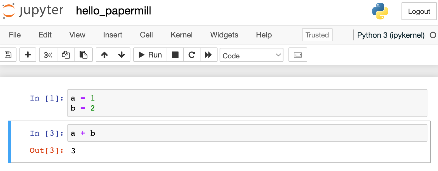
1. Create a Jupyter notebook in your Desktop and name it hello_papermill
2. Say, we want to parameterize a and b to calculate a+b. We will create this code block.

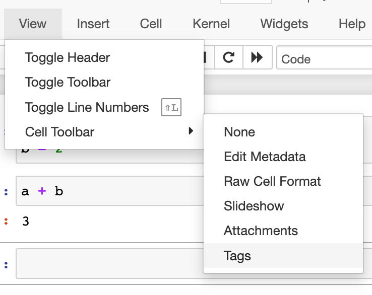
3. Go to the toolbar -> View -> Cell Toolbar -> Tags.

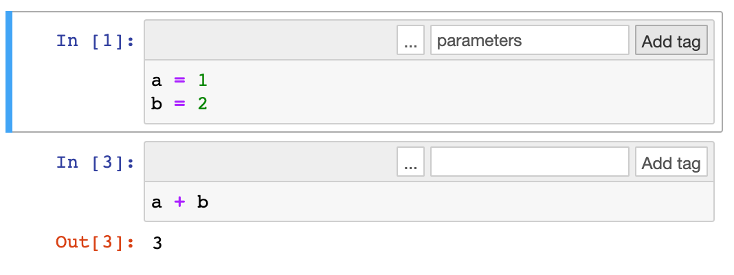
4. Type parametersto top-right corner of the first cell. Click ‘Add tag’. The notebook is parameterized!

5. Start a terminal and navigate to your Desktop.

For Mac users, the command is:

cd ~/Desktop/

For Windows users, the command is

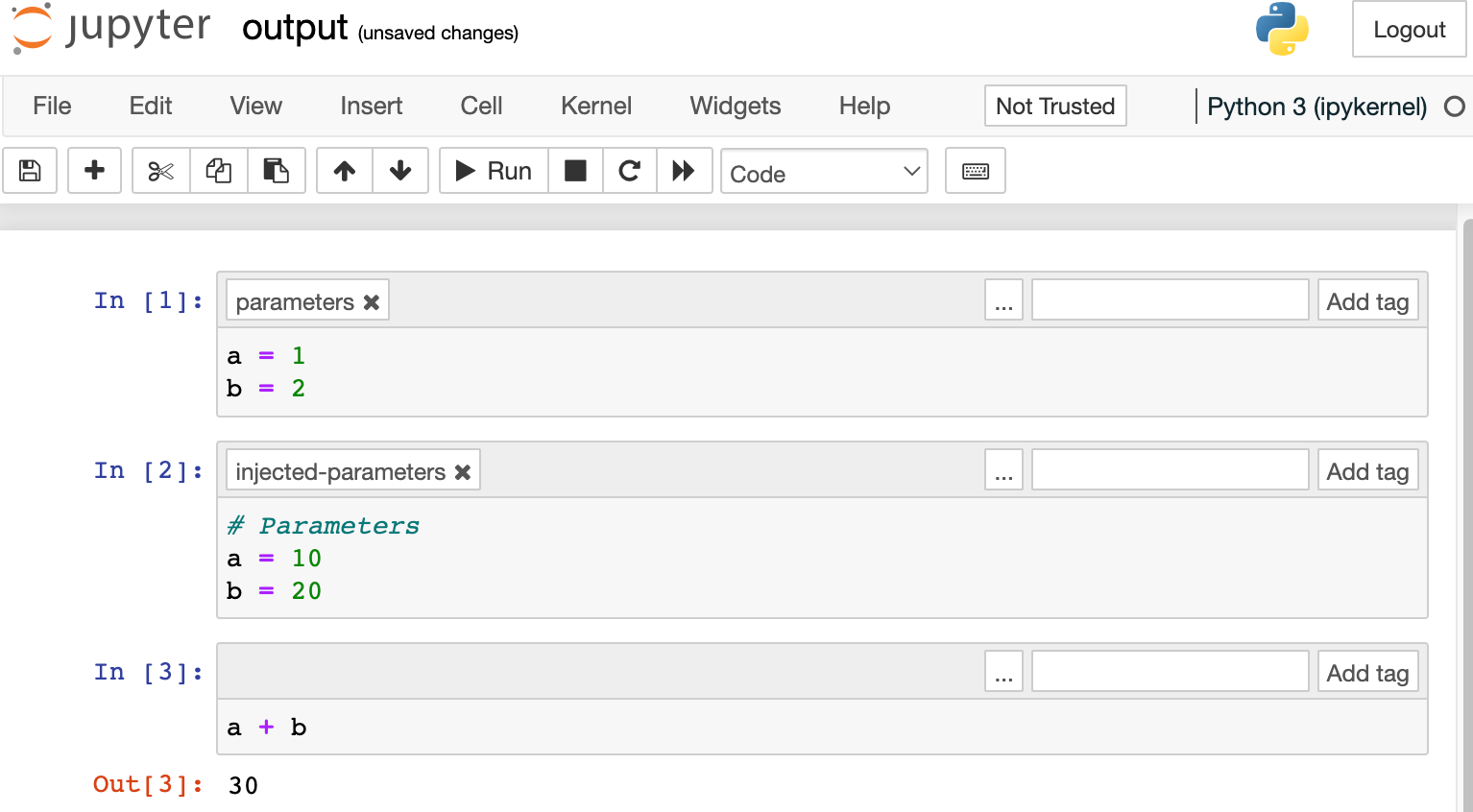
cd C:\Users\YOUR_USER_NAME_HERE\Desktop

6. Run your parameterized notebook with this command. This command tells Papermill to “run hello_papermill.ipynb with the parameters a=10and b=20 and store the results in output.ipynb”

papermill hello_papermill.ipynb output.ipynb -p a 10 -p b 20

7. From the Jupyter interface, open up the output.ipynb. You should see the following automatically generated.

3. Generate a visualization report regularly with Papermill

Now that we have run through the “hello world” of Papermill, let’s dive into the first possible use case.

Before running this code, install the following packags.

pip install yfinance
pip install matplotlib

On my Desktop, I created a Jupyter notebook called plot_stock_price.

This notebook:

• takes in the parameter stock , which is the ticker of the company (MSFT for Microsoft, TSLA for Tesla and Meta for Meta),
• extracts the stock price of a company,
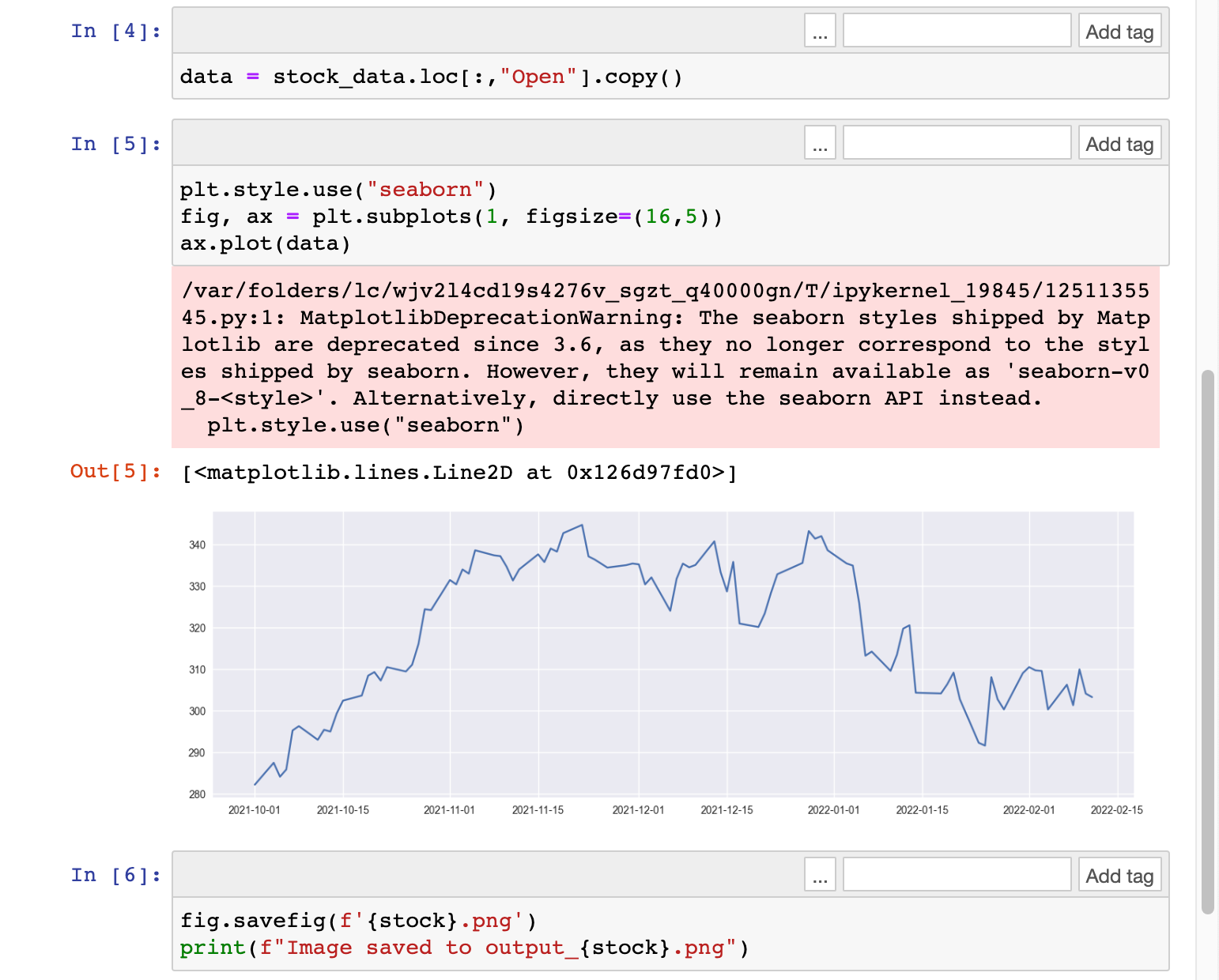
• plots a graph,
• exports the graph as a file named as output_{stock}.png

Here is the code.

import pandas
import yfinance
import matplotlib.pyplot as plt

# selecting a stock ticker
stock = 'MSFT' # This line is parameterized.
stock_list = [stock]

# downloading the stock
stock_data = yfinance.download(stock,start="2021-10-01", end="2022-02-14")
stock_data.head(5)

# plot only the Opening price of ticket
data = stock_data.loc[:,"Open"].copy()

# Plot the data with matplotlib
plt.style.use("seaborn")
fig, ax = plt.subplots(1, figsize=(16,5))
ax.plot(data)

# Save the image as a PNG file
fig.savefig(f'output_{stock}.png')
print(f"Image saved to output_{stock}.png")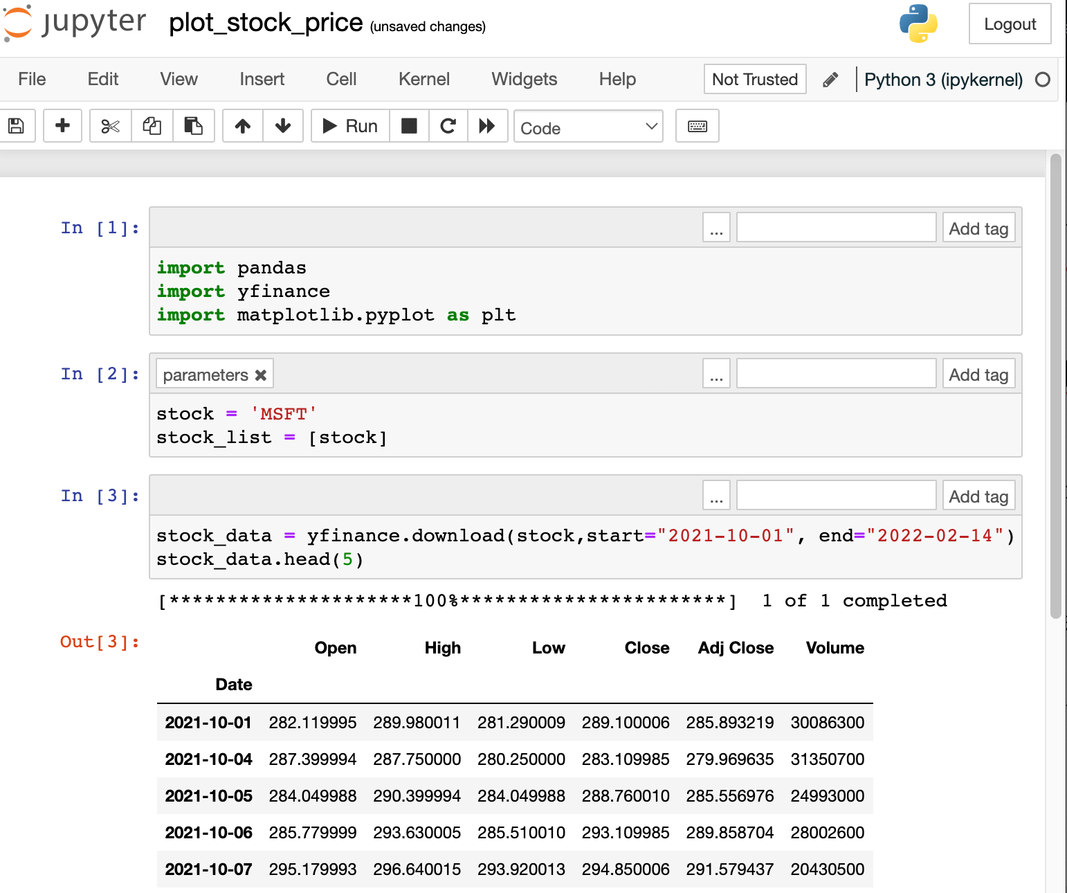

Next, again, open up your terminal and navigate to your Desktop. (I provided some instructions above). Run this command. This tells papermill to “run plot_stock_price.ipynb with the parameter stock='TSLA' and store the output notebook to output.ipynb”.papermill plot_stock_price.ipynb output_TSLA.ipynb -p stock 'TSLA'

You should see something like this in your terminal.

Finally, check your Desktop again. You should see two files: output_TSLA.ipynb and output_TSLA.png . Great, we have successfully ran a parameterized notebook.

4. Run predictions on a trained machine learning on different datasets

The next use case is a familiar one.

You have already trained your machine learning algorithm in a notebook. Now you need to run the algorithm against new data regularly.

Before running this code, install the following packages.

pip install scikit-learn
pip install pandas
pip install numpy

On my Desktop, I created a Jupyter notebook called predict_linear_regression.

This notebook

• trains a linear regression model based on mock data,
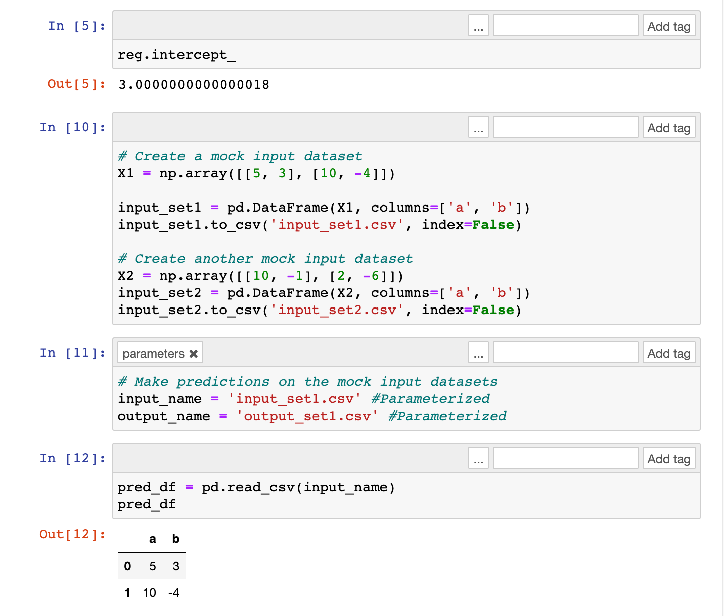
• reads in an input file (CSV) format as a parameter,
• creates mock inputs,
• makes predictions based on inputs in the CSV file, and
• exports the predictions as a file named as output_{stock}.png

import numpy as np
from sklearn.linear_model import LinearRegression
import pandas as pd

X = np.array([[1, 1], [1, 2], [2, 2], [2, 3]])

# Convert the array X into a pandas dataframe
train_df = pd.DataFrame(X, columns=['a', 'b'])

# Create a new column 'y' with the formula y = 3 + a + 2*b 
np.random.seed(5)
train_df['y'] = 3 + train_df['a'] + 2*train_df['b'] 

reg = LinearRegression().fit(train_df.drop(columns=['y']), 
                             train_df['y'])

# Create a mock input dataset 
X1 = np.array([[5, 3], [10, -4]])
input_set1 = pd.DataFrame(X1, columns=['a', 'b'])
input_set1.to_csv('input_set1.csv', index=False)

# Create another mock input dataset
X2 = np.array([[10, -1], [2, -6]])
input_set2 = pd.DataFrame(X2, columns=['a', 'b'])
input_set2.to_csv('input_set2.csv', index=False)

# Make predictions on the mock input datasets
input_name = 'input_set1.csv' # Parameterized
output_name = 'output_set1.csv' # Parameterized

# Read test input
pred_df = pd.read_csv(input_name)

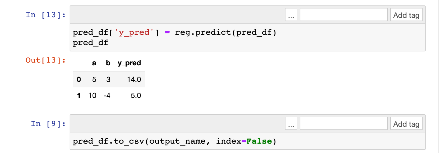
# Make predictions 
pred_df['y_pred'] = reg.predict(pred_df)

pred_df.to_csv(output_name, index=False)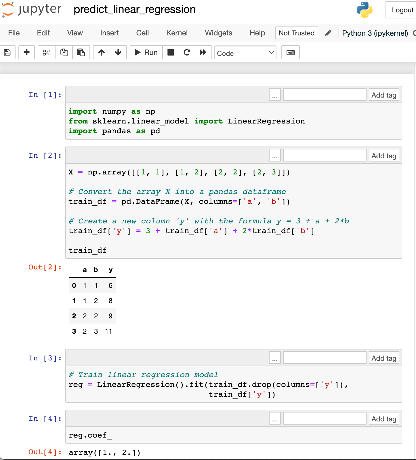

Next, again, open up your terminal and navigate to your Desktop. (I provided some instructions above). Run this command. This tells papermill to “run predict_linear_regression.ipynb with the parameter input_name='input_set2.csv' and output_name ='output_set2.csv' . At the end, store the output notebook to predict_output.ipynb”.

papermill ./predict_linear_regression.ipynb ./predict_output2.ipynb -p input_name './input_set2.csv' -p output_name './output_set2.csv'

You should see something like this in your terminal.

Input Notebook:  ./predict_linear_regression.ipynb
Output Notebook: ./predict_output2.ipynb
Executing:   0%|                                                                                                                                         | 0/11 [00:00<?, ?cell/s]Executing notebook with kernel: python3
Executing: 100%|████████████████████████████████████████████████████████████████████████████████████████████████████████████████████████████████| 11/11 [00:05<00:00,  2.12cell/s]

Finally, check your Desktop again. You should see two files: predict_output2.ipynb and output_set2.csv. Great, we have successfully run a parameterized notebook for a machine learning use case.

5. Do More with Papermill

There are more useful functionalities of Papermill. Here I highlight a few interesting uses.

Running notebooks as functions

Instead of executing the notebook in the terminal, you can execute the notebook as a function. Here are two alternatives that achieve the same goal.

Alternative 1: In terminal, navigate to the directory containing predict_linear_regression.ipynb. Then, run the command

papermill ./predict_linear_regression.ipynb ./predict_output2.ipynb -p input_name './input_set2.csv' -p output_name './output_set2.csv'

Alternative 2: In Jupyter, navigate to the directory containing predict_linear_regression.ipynb. Create a new notebook there and run the command.

import papermill as pm

pm.execute_notebook(
   'predict_linear_regression.ipynb',
   'predict_output2.ipynb',
   parameters = {'input_name': './input_set2.csv', 
                 'output_name': './output_set2.csv')

Upload your results to Amazon S3 or cloud

$ papermill predict_linear_regression.ipynb s3://bkt/output.ipynb -p alpha 0.6 -p l1_ratio 0.1

Provide a .yml file instead of a parameter.

$ papermill predict_linear_regression.ipynb s3://bkt/output.ipynb -f parameters.yaml

6. More resources for Papermill

• Netflix published how they use Papermill to automatically execute notebooks daily for data analytics and engineering work.
• Read the documentation for a clearer idea of how it works.

In this blog post, we have learnt how to parameterize a notebook with Papermill. It’s an excellent tool for optimizing your data science workflow. Give it a try!

I am Travis Tang, a data scientist working in tech. I publish blog posts on TowardsDataScience on open-sourced libraries. On a daily basis, I post data science tips on LinkedIn. Follow me for more regular updates.