Learn Data Science Now: Probability Models

Probability is not the easiest topic to master as its theoretical nuances can be esoteric and arguably obscure. I found a lot of resources online difficult to understand or lacking in rigour — but it need not be that way.

This is why I started this series to explain probability intuitively with easy examples.It’s bite-size data science that you can learn now in 5 minutes.

In this post, I will be using my favourite TV couple, Michael and Jan, as examples. Stay tuned.

This series will be in cover—

1. Probability Models and Axioms (you’re here!)
2. Probability vs Statistics
3. Conditional Probability

Let’s get started!

Probabilistic models

Welcome to lesson 1. Before we dive into any concepts of probability, we need to know what is probability model.

Probability model is simply a way of ascribing chances to events that may or may not happen.

More concretely, a probabilistic model is a mathematical description of an uncertain situation, like the chance of a baby horse being born white when its parents are of different colours.

In probability, we see each uncertain situation as an ‘experiment’ which will have one out of several possible outcomes. The set of all possible outcomes is the sample space of the experiment, while the subset of the sample space is called an event.

The law of probability is simple and elegant. It simply states that the probability of an event must follow the following probability rules, or what we call ‘axioms.’

1. The probability of an event A must not be negative, P(A) ≥ 0
2. If events A and B are disjoint events, then the probability of their union satisfies. Mathematically, P(A ∪ B) = P(A) + P(B)
3. The probability of the entire sample size is equal to one, i.e. P(Ω) = 1

From these three axioms of probability, we can derive many properties of the probability law.

For example, we can derive that the probability of an impossible event is zero from these three axioms. Try it out!

Discrete Uniform Probability Law

We can also derive that the discrete uniform probability law, which states that if n possible outcomes equally likely, then the probability of any event A is P(A) = (Number of event A occurring in n possible outcomes) / n.

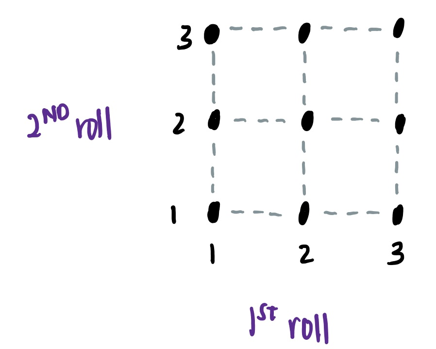
For example, consider rolling a 3-sided coin for 2 times. There are 9 possible outcomes, as shown on the left.

Now, let’s consider the event A that that the rolls are equal to one another. There are three outcomes which fulfills this event, i.e. when both rolls are 1, 2 or 3.

To calculate the probability of event A, we count number of times event A occurs and divide it by the number of possible outcomes.

As such, the P(A) = 3/9 = 1/3.

Simple, right?

Continuous Uniform Probability Law

The discrete uniform probability law applies when the outcome of the experiment is discrete, like rolling a 5 on a die. However, it does not apply when the outcome of an experiment is continuous, like time or the position of a dart throw on a board.

We can similarly define a uniform probability law for continuous outcomes. Under this law, we assign a probability of b-a to any subinterval [a,b] within [0,1].

This can be illustrated with the following examples between Jan and Michael.

Jan is late…

For instance, Michael has a date with Jan but Jan is late. Let’s assume that Jan will arrive anytime within the next 30 minutes with equal probability. This can be represented pictorially using the following diagram called the probability density function.

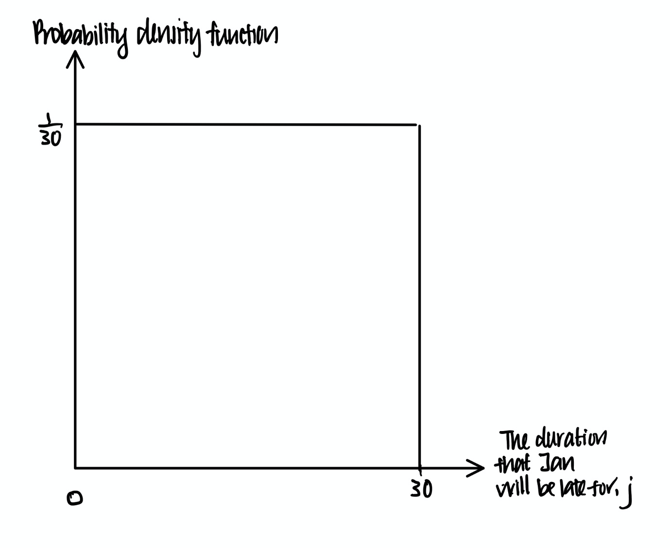
If we see continuous outcome as a line with a length, the probability density function can be seen as ‘probability of unit length’ colloquially. In other words, the product of probability density function and ‘length’ or the event gives us the probability of the event.

Therefore, if we plot a graph of probability density function against ‘length’ of the event, then the area under this graph will be the probability of the event.

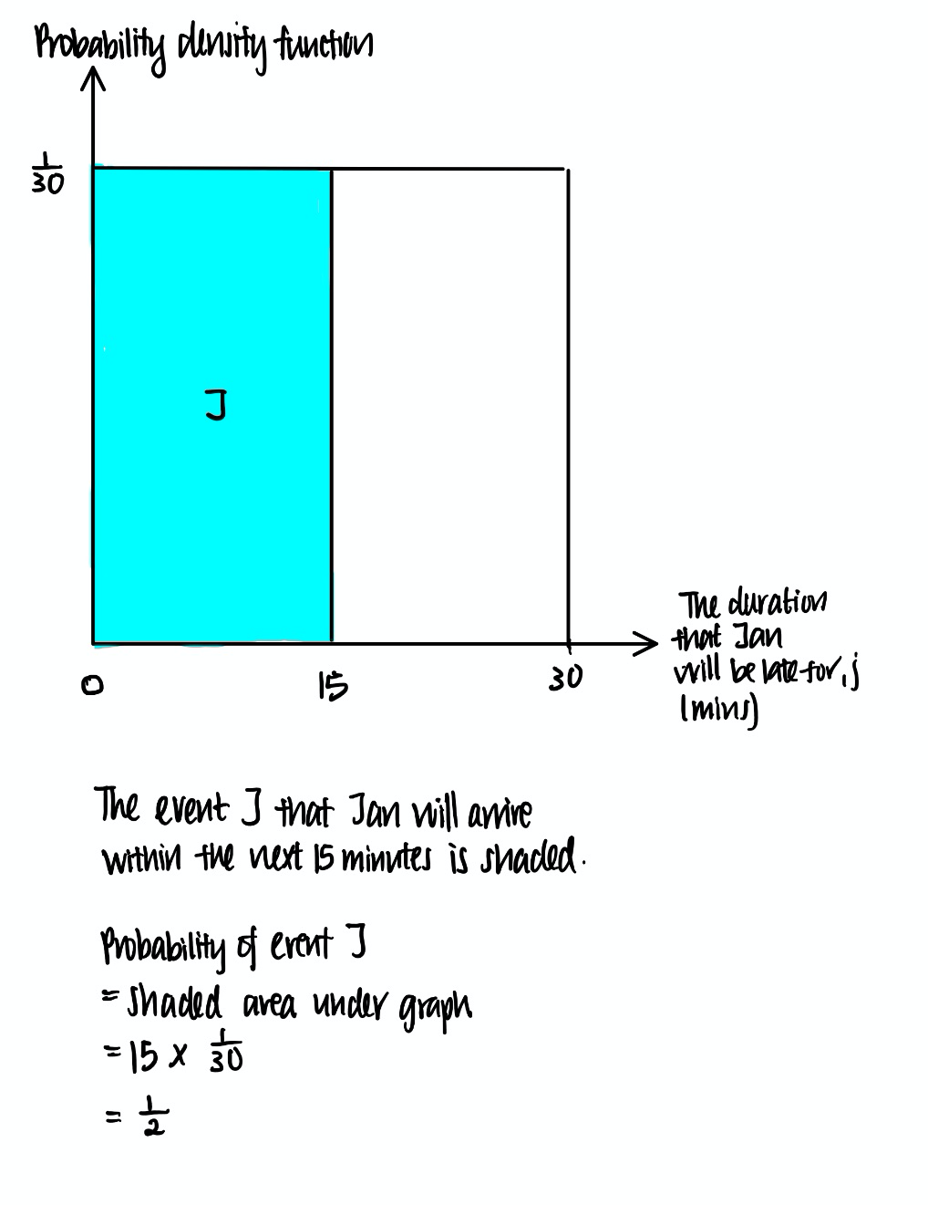
For example, continuing on the previous example, what is the probability that Jan will arrive in the next 15 minutes, assuming that she will arrive anytime within the next 30 minutes with equal probability? This can be represented pictorially as follows.

Jan and Michael are late…

Now, let’s take it a little further. Michael has a date with Jan at 5pm at Chilli’s. Each will arrive at Chilli’s with a delay of between 0 and 1 hour. All pairs of delays are equally likely. The first to arrive will wait for 0.5 hour before leaving angrily.

What is the probability that they will meet?

We know certainly that each will arrive at Chilli’s within 1 hour. As such, we know that this graph contains all events, and this is known as the ‘sample space’.

Now, we want to find out events where they will meet. Let’s think about the different possible scenarios.

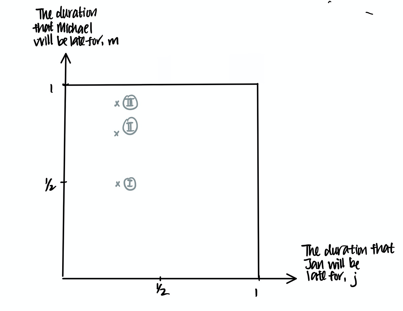
In all scenarios, Jan is late for 15 minutes. In addition, Michael is also late for…

Scenario I. 30 mins (1/2 hour).

Scenario II. 45 minutes (3/4 hour)

Scenario III. 55 minutes respectively.

In Scenarios I and II, Michael arrives within 30 minutes of Jan’s arrival. They meet and have a great time at Chilli’s.

In Scenario III however, Michael arrives 40 minutes after Jan’s arrival. Jan storms off and have a date with Hunter instead.

Now, we can think about all the possible scenarios where Jan and Michael meets. We will eventually realize that the possible scenarios where they meet all fall into the shaded area A in the graph below.

Now, very intuitively, the probability that Michael and Jan meets is simply the area under the graph. With some trigonometry, this works out to be 3/4.

In my next post, I will be focusing on Conditioning and Independence. Stay tuned for more!

To Learn More Probability in Data Science…

I suggest taking the HarvardX Stat 110: Introduction to Probability. This class is by far one of the most rewarding I have attended. Professor Blitzstein, one of my favourite professors for probability, covers the topics rigorously and intuitively.

You can audit the course for free. If you like the class, you can pursue a verified certificate to highlight your knowledge in probability.

Let’s Connect!

I love connecting with data science learners so we can learn together. I post all things data science regularly.